It’s quite some time since we arrived at Riemann’s main result, the explicit formula
\[ J(x)=\mathrm{Li}(x)-\sum_{\Im\varrho>0}\left(\mathrm{Li}(x^\varrho)+\mathrm{Li}(x^{1-\varrho})\right)+\int_x^\infty\frac{\mathrm{d}t}{t(t^2-1)\log t}-\log2, \]
where \(J(x)\) is the prime power counting function introduced even earlier. It’s high time we applied this!
First, let’s take a look at \(J(x)\) when calculating it exactly:
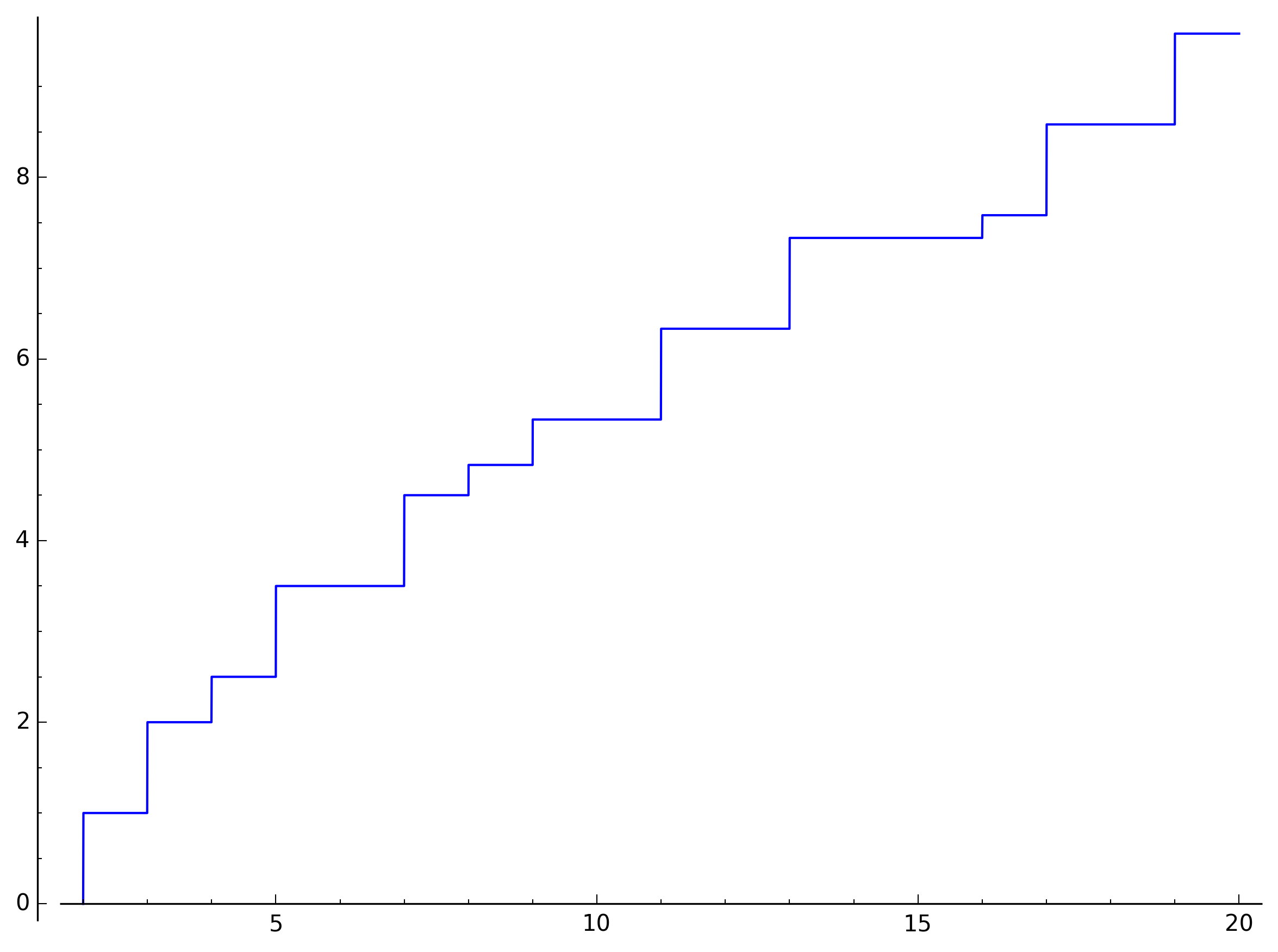
You see how this jumps by one unit at prime values (\(2\), \(3\), \(5\), \(7\), \(11\), \(13\), \(17\), \(19\)), by half a unit at squares of primes (\(4\), \(9\)), by a third at cubes (\(8\)), and by a quarter at fourth powers (\(16\)), but is constant otherwise.
Now, the point about Riemann’s formula is that if you worked out diligently every single term on the right hand side exactly (and there’s an infinity of smooth functions there) – you’d end up with the same step function I just plotted!
This thought always makes my brain hurt a little, so let’s take it step by step. Of course, it’s impossible to work every term since this would require to know the value of every single zeta zero. Instead, we will look at increasingly better approximations as we add more and more zeros into the equation. Let start from what it looks like when we only use the terms without the zeta zeros, i.e., \(\mathrm{Li}(x)\), \(\log2\), and the integral:
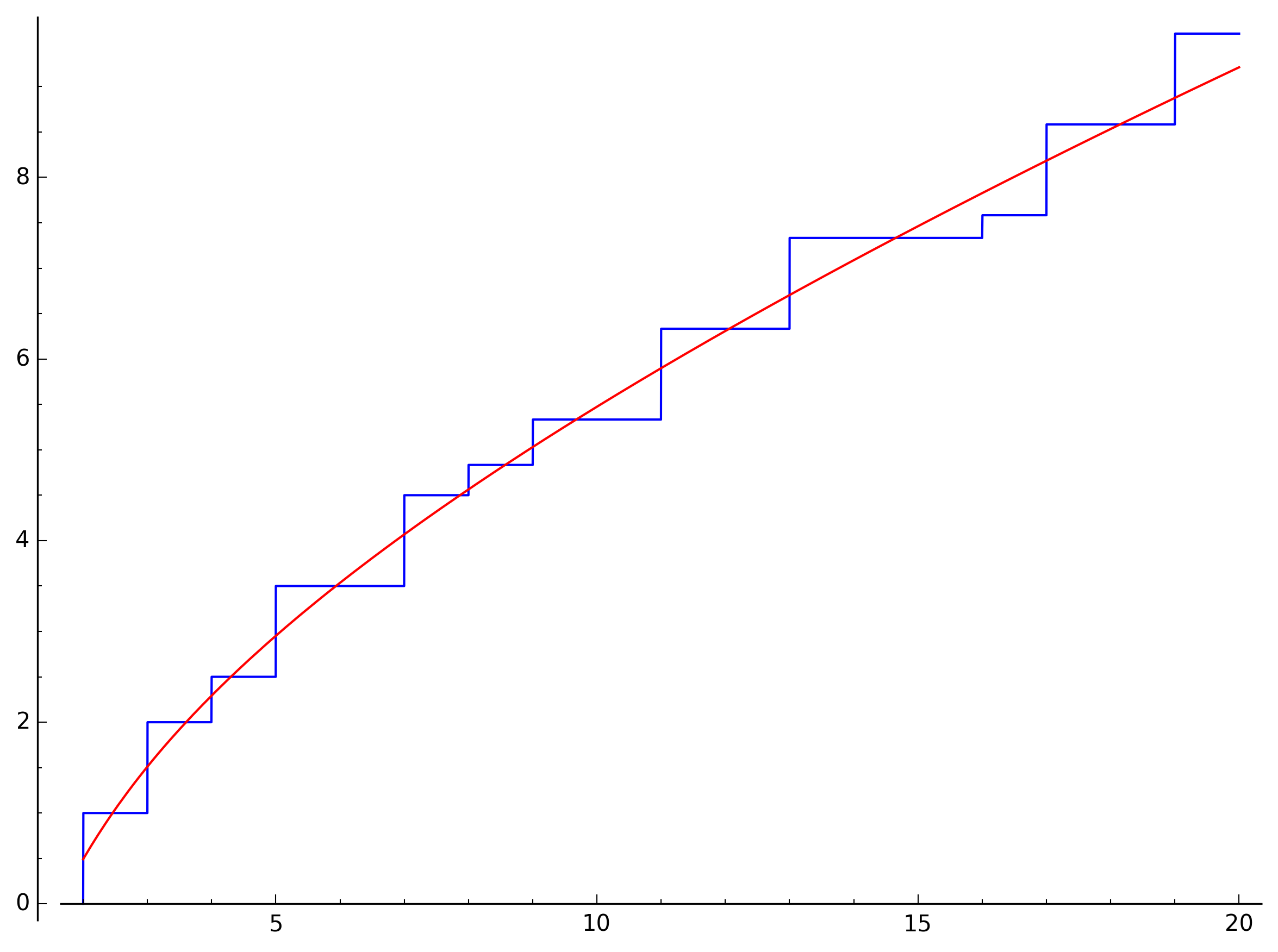
This already looks like a pretty good approximation, but we already do much better by just adding the first three1 zeros:
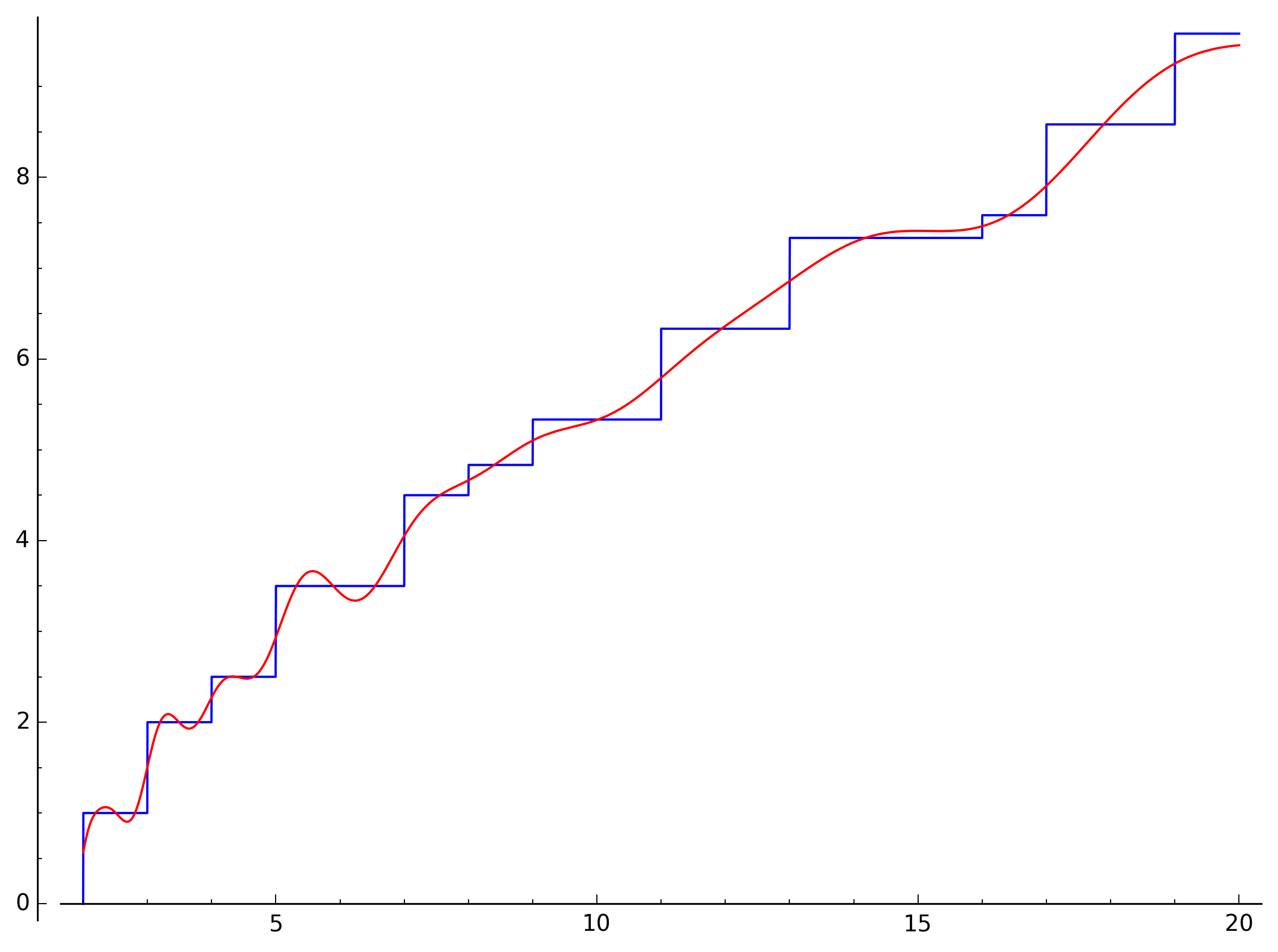
Note how elegantly the previously monotonous function dances in waves around the prime steps. But this is only the start – with ten zeros the waves are getting more dense:
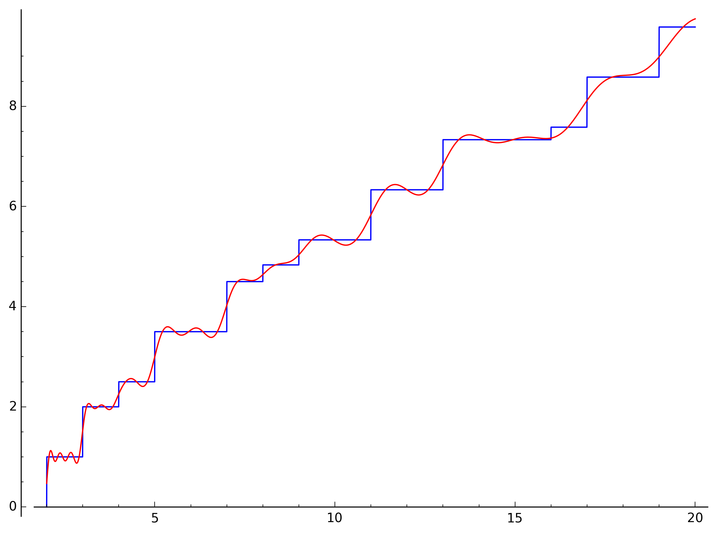
By the time we added one hundred zeros it’s getting pretty hard to distinguish the two functions:
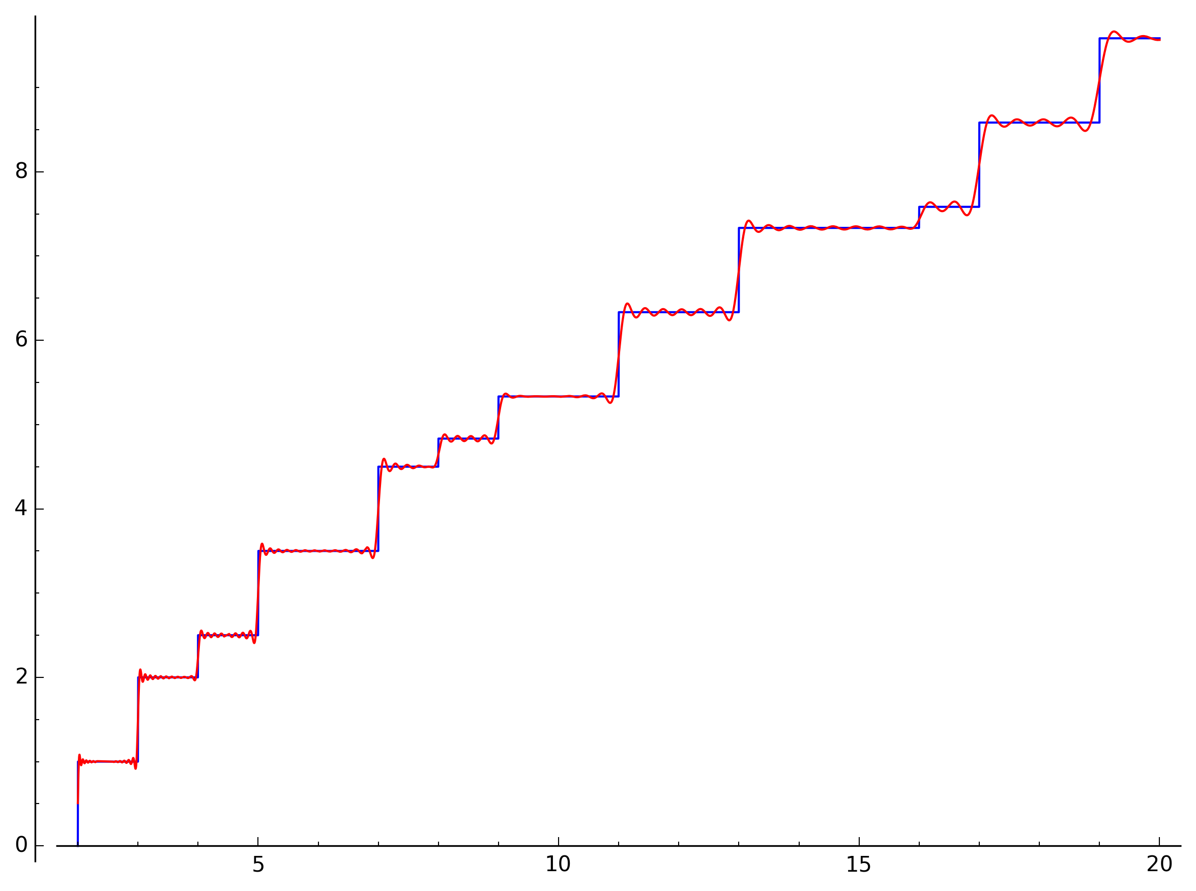
I think you can’t get much closer to seeing the music of the primes!
If you’re worried that we just got lucky with the small values, here’s a plot of the values up to \(200\) with twenty zeros used in the approximation:
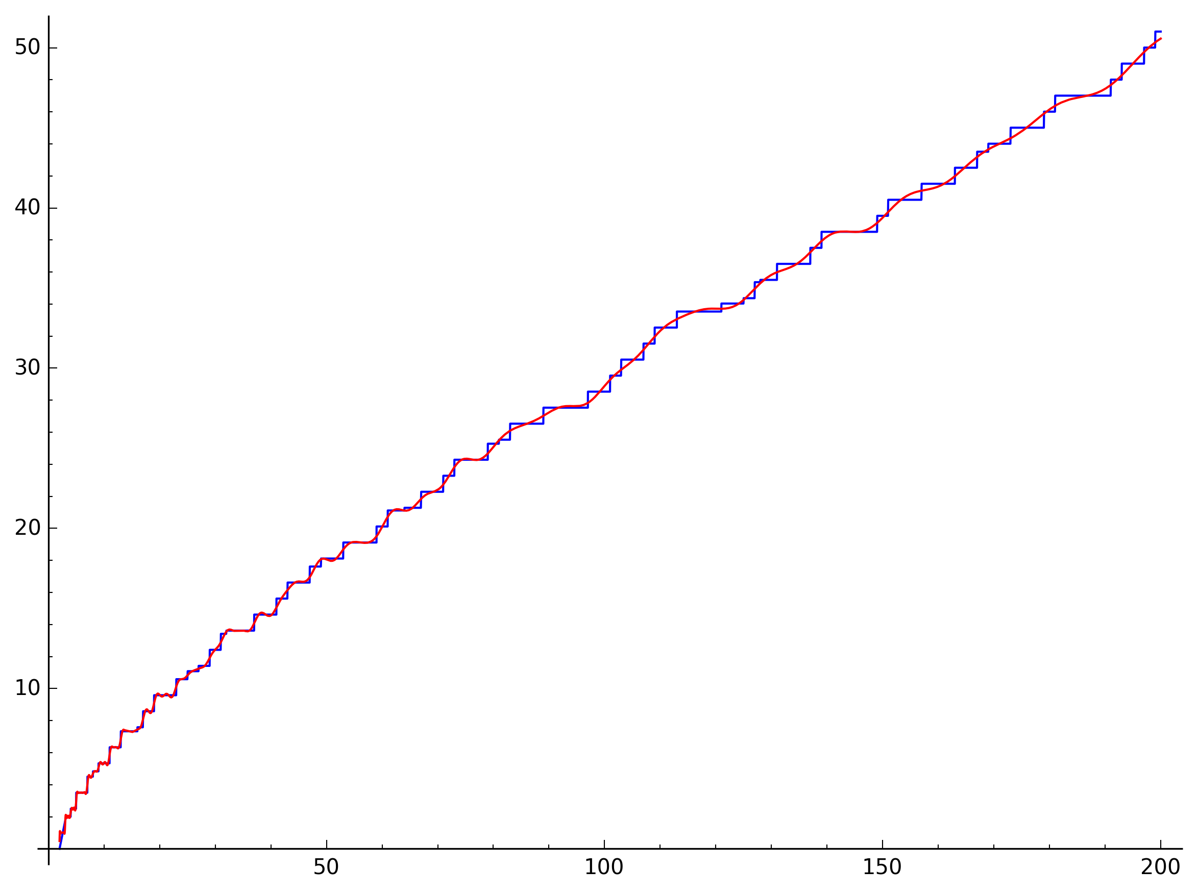
Note what a close match the approximation is for small values of \(x\), but even further up the approximation will never let \(J(x)\) go too far astray.
I could carry on with more plots with higher values of \(x\) or more zeros added, but this would only really look like two identical smooth lines, so the way this works is actually much clearer in smaller values.
I’ll conclude with two thoughts: First, the equation and the pictures are in terms of this somewhat exotic \(J(x)\), but we were really interested in \(\pi(x)\), the number or primes less than \(x\). This is really not a big deal, since we can just apply Möbius inversion to the definition of \(J(x)\) and get back the values of \(\pi(x)\):
\[ \pi(x)=\sum_{n\geq1}\frac{\mu(n)}{n}J(x^{1/n}). \]
Just plug in our approximations for \(J(x)\) and we will get out an approximation for \(\pi(x)\).
Second, the approximations are smooth functions, but our actual objects of study are discrete step functions. In particular, \(\pi(x)\) can only ever take on integer values, which actually helps a lot when doing computations. We don’t need to add more and more zeros to get the precise value of \(\pi(x)\). Instead, as soon as our approximation is zooming in on an integer, this must be the correct value, and we can move on.
That said, calculating the approximation to any degree of accuracy for high values of \(x\) requires precise knowledge of a lot of zeta zeros and even more computing power. In the end, it is much faster just to tabulate the prime numbers and count them directly.
But of course, we are not doing this for a particular practical reason, but to understand prime numbers – and Riemann’s formula gave the researchers of his time finally the tools to prove the Prime Number Theorem.
-
In what follow I always refer to the zeros ordered in increasing height up the critical line plus their respective mirror images with negative imaginary part. ↩︎