Tossing the Prime Coin

One of the problems with explaining the Riemann Hypothesis is that its fascination comes from its deep connection to prime numbers, but its definition is in terms of complex analysis which requires a fair deal of undergraduate mathematics to understand – and that is before you even got started to grasp what the heck the zeta-zeros have to do with the distribution of primes. My “cocktail party explanation” of the Riemann Hypothesis would usually be something like: “The prime numbers are as equally distributed as you could wish for.” But there is actually a surprisingly easy interpretation of the Riemann Hypothesis: “Prime numbers behave like a random coin toss.”

Let’s first take a look at a regular (fair) coin, that is, the two outcomes “heads” or “tails” are equally likely. We now do an experiment: we start counting at \(0\), and toss our coin repeated. Whenever we throw “heads”, we add \(1\) to our count, when it’s a “tails”, we subtract \(1\). What will be the count after \(n\) coin tosses?

Mathematically speaking, we define a sequence of independent random variables \(X_i\) where

\[ P(X_i=1)=P(X_i=-1)=\frac{1}{2}. \]

Now we are interested in what the sum is, i.e., we define

\[ Y_n=\sum_{i=1}^n X_i. \]

Because of the \(X_i\)’s symmetry, they each have \(EX_i=0\), and hence we also have \(EY_n=0\) for all \(n\) (due to the linearity of the expectation value). In other word, if we were to bet on what our total count would be at any given point, we should put our money on \(0\).¹

However, reality looks different.

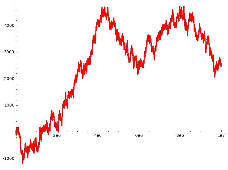
This is an example of how \(Y_n\) might develop. (You see why this process is known as a random walk.) When we stopped at \(n=10^7\), we were off \(0\) by about \(2000\). After all, that shouldn’t be too surprising. In theory, \(Y_n\) could take any value between \(-n\) and \(n\). However, these boundary values would be extremely unlikely: the probability that \(Y_{10^7}=10^7\) is indeed \(2^{-10^7}\), a ridiculously small number.

Still, despite its tendency to oscillate around the \(x\)-axis, we would observe that \(Y_n\) would reach arbitrary distances from it as \(n\) grows larger and larger. The way to quantify this behaviour is to measure the standard deviation of \(Y_n\). I won’t go into the details, but if you’re familiar with these calculations you won’t have a problem verifying that

\[ \sigma Y_n = \sqrt{\mathrm{Var}Y_n} = \sqrt{E(Y_n^2)-(EY_n)^2} = \sqrt{n-0^2} = \sqrt{n}. \]

This means that while we expect \(Y_n\) to be \(0\) on average, we would expect the values to spread up to \(\sqrt{n}\):

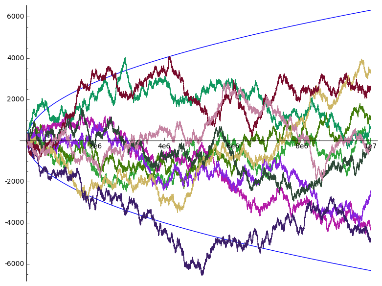
More precisely, we would expect values between \(-1.96\sqrt{n}\) and \(1.96\sqrt{n}\) in \(95\%\) of the cases if we repeated the experiment over and over again. We can visualise this if we take a look at a few more random walks:

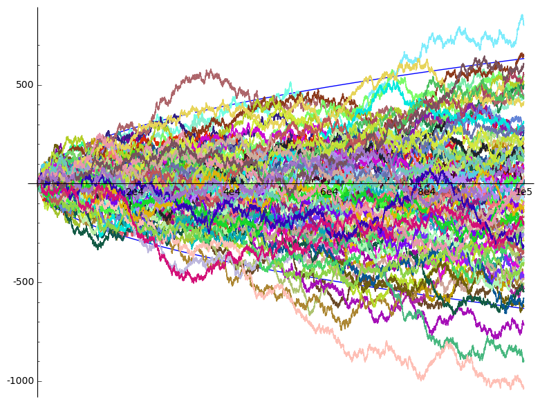
Out of these 100 random walks, indeed 5 ended up outside the square root region.

But for random walks, we can make an even more precise statement. The law of the iterated logarithm asserts that the rate of growth of a random walk is governed by \(\sqrt{n\log\log n}\), so we might say²

\[ Y_n\approx O(\sqrt{n\log\log n}), \]

which of course has to be interpreted with some good will³ since we are talking here about a random sequence, not a deterministic one.

That’s all very well, but what does it have to do with primes or the Riemann Hypothesis? To see this, we need to remember the Möbius function \(\mu(n)\) that I half-heartedly introduced some time ago. The definition of this function looks very odd and artificial at first, but is actually a very natural and useful function in the theory of numbers, not least because of the Möbius inversion mentioned in the article above. We define \(\mu(n)\) as follows: if \(n\) has \(k\) prime factors, all of which are distinct (i.e., \(n\) is squarefree), then \(\mu(n)=(-1)^k\), otherwise, if \(n\) has at least one repeated prime factor, \(\mu(n)=0\). The sequence \(\mu(n)\) looks like this:

\[ \mu=1,-1,-1,0,-1,1,-1,0,0,1,-1,0,-1,1,1,0,-1,0,-1,0,\ldots \]

Notice how \(\mu(p)=-1\) for primes \(p\) since they have exactly one prime factor (themselves). But there are also composite values with \(\mu(n)=-1\), e.g., \(n=30\). In general, it seems pretty hard to predict what value will come next. The sequence looks random. Of course, it isn’t actually random since the values are predefined by the arguments’ prime factors. It is exactly this unpredictable, yet not erratic nature of the primes that the zeta-zeros encode.

To see what I mean, we’ll sum up the values of \(\mu(n)\) just like we did with out coin tosses. The result

\[ M(n)=\sum_{k=1}^n\mu(k) \]

is called the Mertens function, and looks like this:

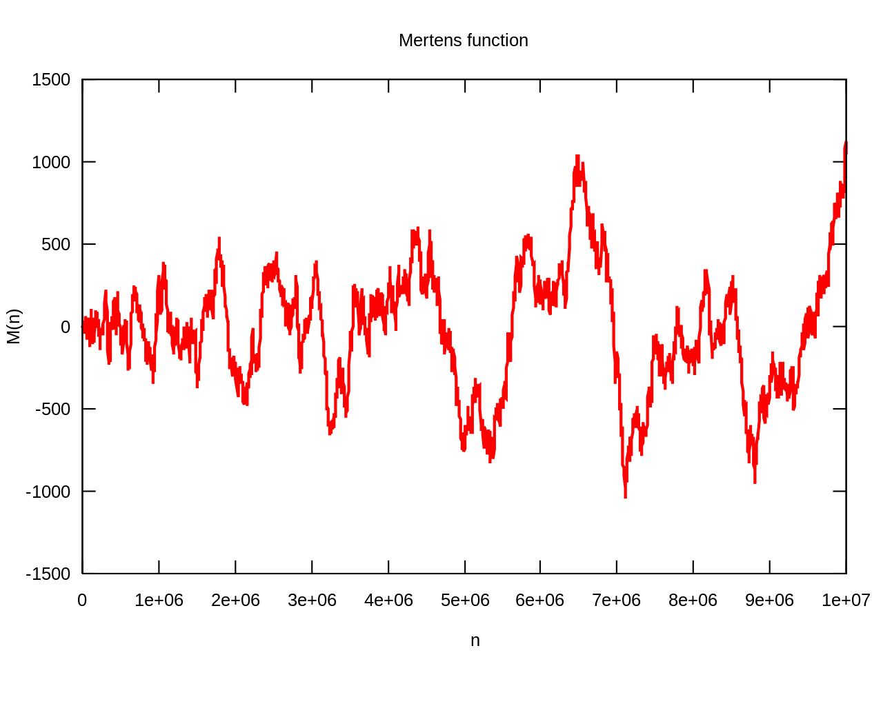
From this (small) sample, \(M(n)\) looks pretty much like one of our random walks. One crucial difference however is that about \(40\%\) of the values are \(0\). (More precisely, the proportion of squarefree numbers amongst all integers converges to \(6/\pi^2\) which may look familiar to you as the value of \(1/\zeta(2)\), but this deserves an article of its own.) To get a better comparison we’ll just skip these values in our “random prime walk”: If we take the values of \(\mu\), can we distinguish the resulting sequence of \(1\) and \(-1\) from a sequence of random coin tosses? A small comparison actually makes it look like \(\mu(n)\) is rather better behaved than a coin toss (the prime walk is overlaid in red):

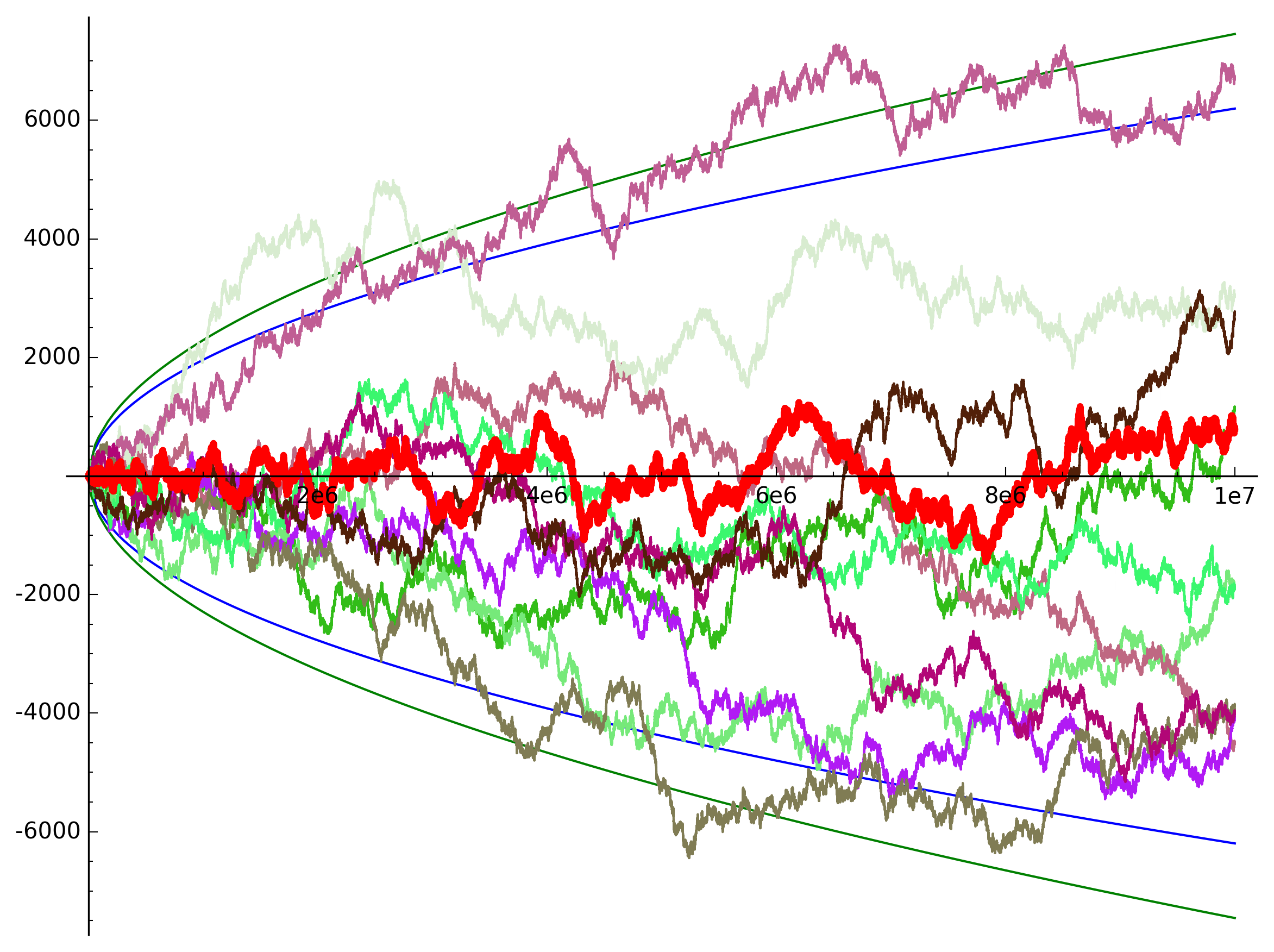
Since this is not actually a random variable, we cannot talk of expectation values or standard deviations, but we can control its rate of growth. If \(M(n)\)⁴ really behaved like a random walk, we would expect it to be delimited by the square root function, and indeed did Franz Mertens conjecture the stronger statement that \(|M(n)|<\sqrt{n}\) for all \(n\). This turned out to be wrong⁵, but not all is lost – after all, we don’t have such a tight bound on our coin tosses either. Instead, we would be happy with something like

\[ M(n)=O(n^{1/2+\varepsilon}). \]

This indeed is equivalent to the Riemann Hypothesis. To see this, we first observe that

\[ \sum_{n\ge1}\mu(n)n^{-s}=\frac{1}{\zeta(s)}. \]

(There are many clever ways to see this, but you will have to trust me on this – or, much better, verify it yourself.) Through a clever sequence of transformations, we express \(M(n)\) as an integral, and then get it out of it via Mellin transform to obtain

\[ M(x) = \frac{1}{2 \pi i} \int_{\sigma-i\infty}^{\sigma+i\infty} \frac{x^s}{s \zeta(s)} \mathrm{d}s. \]

The crucial question is for what values of \(\sigma\) this is valid. We will change the value of the integral if we push the line of integration to the left past a singularity in the integrand. This will happen if there is a zero in the denominator. Voilà, the zeta-zeros entered the stage!

If Riemann was right, there will be no zeros for \(\Re\sigma>\frac{1}{2}\), and hence we could choose \(\sigma\) to be as little as \(\frac{1}{2}+\varepsilon\) (where \(\varepsilon>0\) is an arbitrarily small number). But then it is not difficult to convince yourself⁶ that this implies \(M(n)=O(n^{1/2+\varepsilon})\), just as we were hoping for.

In other words: if the Riemann Hypothesis is true, then the sequence \(M(n)\) is very close (though not quite) to looking like a random walk. What’s more is that the converse is true as well, i.e., you could deduce the Riemann Hypothesis from the above bound for \(M(n)\): if Riemann is false, then there are zeros off the critical line and we will know that the Mertens function has a wider spread than a random walk. That’s why we say that these statements are equivalent.

So when someone asks you next time how it is to work on primes, just say that it’s like flipping a coin – you never know what you’ll get.

See also

• How NOT to Earn a Million Dollars